Tracking Metrics for Monado
Mateo de Mayo
21 March 2022
Summary
This post presents what is now possible after a couple of updates that allow Monado to analyze SLAM trackers and datasets in batch to assess their performance and accuracy, thus giving an objective idea of whether the tracking is really improving and how good it is working. It is also a good opportunity to present tables that compare the different integrated systems and give you an idea of how well things are working with each fork.
When working with tracking systems it can happen that you wake up one day, and the tracking feels better than the day before without any particular reason to attribute the improvement to. Questions like “maybe the USB connection was a bit loose yesterday?” or even “could it be because today is more sunny?” when using camera-based tracking are some I came to formulate in these scenarios. It could even be the case that you just woke up in a better mood and tolerate tracking issues a bit more.
After realizing this, I figured it was essential to have a good way of objectively determining the performance of a system on a given sequence of datasets. More so considering the next steps with the tracking in Monado include going deeper into the SLAM/VIO systems’ pipelines.
A couple of tools for measuring the accuracy and performance of SLAM systems exist, SLAMBench1 being a very good example, but even then we needed ways of automatizing the process of generating data for evaluation of datasets in Monado. This post tries to summarize what is now possible regarding SLAM/VIO evaluation in Monado.
Generating the data
The first merge request in this line of work was this one. It does a couple of things like allowing the SLAM systems to report their internal pipeline times back to Monado, and integrates into Monado the possibility to use reference trajectories (ground truth) if available from the SLAM sources (e.g., EuRoC dataset player). It enables the possibility to display in real-time both the tracking error2 and the timing information of the systems as seen in the curves to the left of the image below.
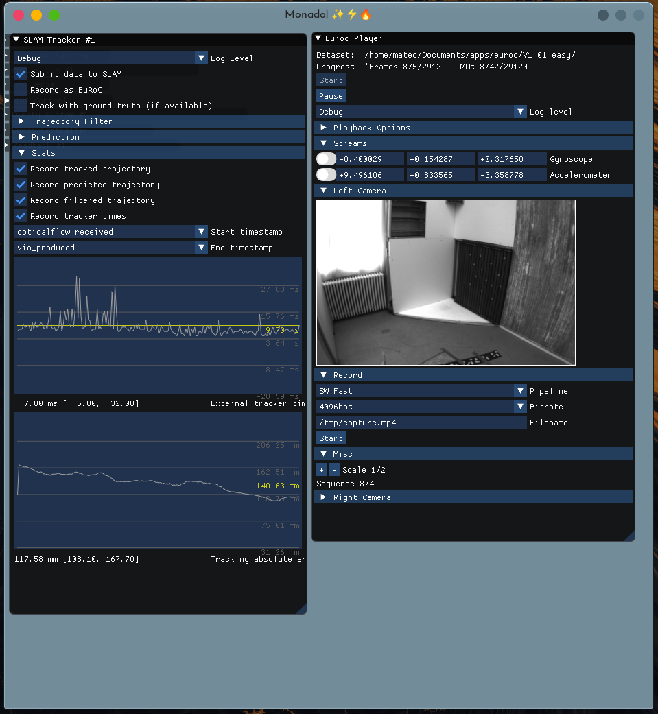
However, the most important thing that that MR introduces is the ability to save CSV files with the timing information and the estimated, predicted and filtered trajectories from the tracker in CSV files for offline analysis like this:
For the predicted poses saved in tracking.csv you have:
# timestamp [ns], p_RS_R_x [m], p_RS_R_y [m], p_RS_R_z [m], q_RS_w [], q_RS_x [], q_RS_y [], q_RS_z []
6997681930473,0.0000000000,0.0000000000,0.0000000000,0.5557456613,0.0009835553,-0.8313517570,0.0000000000
6997731930601,-0.0000058096,-0.0000130947,0.0000100406,0.5557390451,0.0009709296,-0.8313562274,0.0000112125
6997781930473,-0.0000083494,-0.0000609047,0.0000496814,0.5557395816,0.0009258533,-0.8313559294,0.0000084368
6997831930601,0.0000331269,-0.0001313922,0.0001094043,0.5557386875,0.0009122558,-0.8313565254,0.0000182058
6997881930473,-0.0000239215,0.0001417128,-0.0000660935,0.5551946759,0.0003172281,-0.8317196965,0.0010597851
6997931930601,0.0000156540,0.0003277477,0.0001416763,0.5555265546,0.0004448513,-0.8314981461,0.0009185750
6998031930601,0.0000845920,0.0003950795,-0.0000916694,0.5554929376,-0.0000688768,-0.8315203190,0.0012723863
...
While for the timing information saved in timing.csv you get something like:
# frame_ts,tracker_received,opticalflow_received,vio_received,tracker_consumer_received,received_by_monado
6997681930473,6997694542317,6997695262125,6997699258602,6997699631993,6997700087150
6997731930601,6997743955455,6997745236261,6997749067885,6997749198851,6997749938120
6997781930473,6997791383303,6997792716579,6997796591373,6997796698030,6997799916475
6997831930601,6997838933853,6997839698854,6997842708168,6997842804635,6997850212650
6997881930473,6997888078063,6997888855419,6997891708941,6997894958478,6997899706131
6997931930601,6997936733173,6997937138050,6997940231291,6997942182912,6997949933197
6997981930473,6997986854881,6997987260573,6997989946485,6997992114463,6998000756394
6998031930601,6998036722866,6998037490713,6998040232329,6998042449818,6998050688152
6998081930473,6998086709312,6998087110536,6998089822441,6998091790862,6998101053875
You also get prediction.csv and filtering.csv which correspond,
respectively, to the predicted and filtered trajectories the tracker returns to
the XR app.
Generating it in bulk
The next merge
request
introduces the monado-cli slambatch command. This command allows Monado to run
multiple datasets at once to generate all of these CSV files for each and is
designed to run without UI so that it’s CI friendly. You can run a command like:
monado-cli slambatch \
  $euroc/MH_04_difficult $bsltdeps/basalt/data/monado/euroc.toml MH04 \
  $euroc/V1_02_medium $bsltdeps/basalt/data/monado/euroc.toml V102 \
  $tumvi/dataset-room3_512_16 $bsltdeps/basalt/data/monado/tumvi.toml R3
And then you obtain the respective CSV files:
.
├── MH04
│   ├── filtering.csv
│   ├── prediction.csv
│   ├── timing.csv
│   └── tracking.csv
├── R3
│   ├── filtering.csv
│   ├── prediction.csv
│   ├── timing.csv
│   └── tracking.csv
└── V102
    ├── filtering.csv
    ├── prediction.csv
    ├── timing.csv
    └── tracking.csv
Analyzing the data
Finally, a set of python scripts were written in the xrtslam-metrics repo
that are designed to analyze all of this data programmatically.
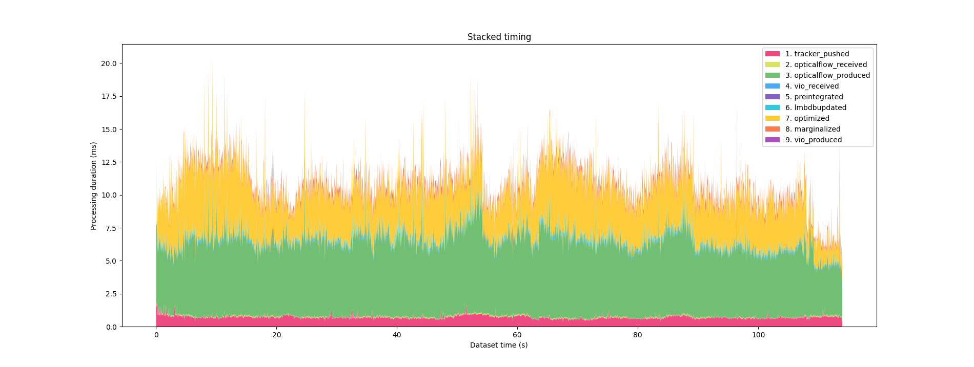
For analyzing the processing times, you can specify the start and end columns
(i.e., pipeline stages) in timing.csv that you are interested in analyzing like this:
$ ./timing.py runs/BNF/EV201/timing.csv tracker_pushed vio_produced -p
TimingStats(mean=10.13590801754386, std=1.895429240022987, min=4.155935, q1=9.018804, q2=10.062223, q3=11.3165765, max=19.492825) from 'tracker_pushed' to 'vio_produced'
And a plot like this is produced:
Some systems are not stable enough to complete all dataset before crashing and
so completion.py can tell you what’s the percentage it gets to complete.
$ ./completion.py runs/K/TR1/tracking.csv targets/TR1/cam0.csv
|:---------------------|:--------|
| Groundtruth poses    | 2821    |
| Estimated poses      | 268     |
| Tracking duration    | 56.75s  |
| Groundtruth duration | 141.00s |
| Tracking completion  | 40.25%  |
Then you have the accuracy statistics, both in terms of absolute (ATE) and
relative (RTE) trajectory errors, which are standard in the field and are the
ones you will encounter in the systems papers. For this xrtslam-metrics uses
the awesome EVO library. It’s worth
noticing that each paper implements this statistics just a bit different, my
decisions here tries to align with what makes more sense for XR.
$ ./tracking.py ate targets/EV201/gt.csv runs/BNF/EV201/tracking.csv
APE w.r.t. translation part (m)
(with SE(3) Umeyama alignment)

       max	0.073318
      mean	0.035746
    median	0.034026
       min	0.006925
      rmse	0.038935
       sse	3.395612
       std	0.015432

$ ./tracking.py rte targets/EV201/gt.csv runs/BNF/EV201/tracking.csv -p
RPE w.r.t. translation part (m)
for delta = 6 (frames) using consecutive pairs
(with SE(3) Umeyama alignment)

       max	0.015671
      mean	0.002855
    median	0.002477
       min	0.000116
      rmse	0.003472
       sse	0.004496
       std	0.001976
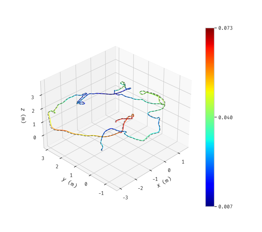
These also allow you to produce figures with the -p flag to compare the
trajectory to the ground truth in 3D.
Furthermore, you can use the entirety of tools offered by EVO on the
tracking.csv files from the CLI to compare specific trajectories. You can see
what’s possible in the EVO home page.
And last but not least, batch.py allows you to generate markdown tables out of all runs!
Cells are mean ± stdev of the entire run. See below the tables an explanation of what each row and column means.
Processing times [ms]
| BND | BNF | BO | K | ON | OO | |
|---|---|---|---|---|---|---|
| C6EASY | 826.60 ± 441.30 | 5.84 ± 1.38 | 9.05 ± 2.40 | 46.00 ± 6.10 | 36.11 ± 7.67 | 35.09 ± 11.81 |
| C6HARD | 668.75 ± 555.59 | 5.58 ± 1.38 | 9.83 ± 3.01 | 47.45 ± 7.94 | 30.66 ± 9.64 | 32.92 ± 12.41 |
| C8EASY | 940.54 ± 485.31 | 6.93 ± 2.10 | 12.89 ± 13.63 | 49.23 ± 7.37 | 33.69 ± 10.50 | 33.24 ± 10.22 |
| C8HARD | 716.58 ± 579.89 | 6.20 ± 2.46 | 12.60 ± 8.38 | 46.28 ± 7.89 | 35.83 ± 11.75 | 37.43 ± 12.04 |
| COEASY | 873.74 ± 404.36 | 6.17 ± 1.12 | 10.96 ± 2.94 | 37.25 ± 4.94 | 35.40 ± 9.35 | 29.41 ± 9.69 |
| 734.47 ± 357.71 K | 6.24 ± 1.02 K | 10.92 ± 2.98 K | ||||
| COHARD | 617.47 ± 419.17 | 5.71 ± 1.16 | 12.90 ± 3.83 | 37.31 ± 5.20 | 21.52 ± 7.61 | 23.69 ± 7.98 |
| 592.62 ± 410.55 K | 5.81 ± 1.02 K | 12.81 ± 3.81 K | ||||
| EMH01 | 2123.22 ± 1118.05 | 10.63 ± 3.22 | 14.17 ± 3.15 | 53.15 ± 7.00 | 30.29 ± 6.63 | 36.73 ± 12.68 |
| EMH02 | 2280.38 ± 1118.44 | 11.16 ± 4.28 | 15.33 ± 5.76 | 53.93 ± 6.05 | 29.29 ± 5.37 | 35.32 ± 10.40 |
| EMH03 | 2184.08 ± 940.11 | 11.02 ± 2.81 | 15.17 ± 3.65 | 53.83 ± 6.05 | 32.09 ± 5.71 | 37.08 ± 12.91 |
| EMH04 | 2117.07 ± 916.61 | 11.82 ± 3.73 | 15.83 ± 3.41 | 53.12 ± 7.19 | 29.77 ± 6.94 | 32.67 ± 11.86 |
| EMH05 | 2187.28 ± 902.72 | 11.17 ± 2.15 | 15.47 ± 3.63 | 53.40 ± 7.07 | 29.04 ± 6.17 | 34.06 ± 15.61 |
| EV101 | 1687.89 ± 524.66 | 10.23 ± 1.76 | 13.62 ± 2.21 | 54.37 ± 6.18 | 30.26 ± 5.95 | 35.43 ± 13.93 |
| EV102 | 1322.72 ± 624.59 | 10.18 ± 2.09 | 15.35 ± 3.63 | 55.48 ± 5.79 | 29.74 ± 6.06 | 32.71 ± 13.47 |
| EV103 | 844.55 ± 609.03 | 11.65 ± 2.56 | 17.31 ± 4.37 | 56.54 ± 6.47 | 34.74 ± 11.43 | 31.13 ± 10.70 |
| EV201 | 1628.73 ± 718.45 | 10.08 ± 1.89 | 15.53 ± 3.04 | 55.00 ± 5.66 | 36.63 ± 11.87 | 32.51 ± 10.04 |
| EV202 | 1296.74 ± 667.75 | 10.65 ± 3.49 | 17.57 ± 4.14 | 55.37 ± 5.24 | 37.77 ± 10.90 | 34.78 ± 11.45 |
| TR1 | 800.61 ± 327.45 | 6.37 ± 1.02 | 12.54 ± 2.70 | 21.34 ± 3.51 | 46.72 ± 11.81 | 44.95 ± 12.33 |
| TR2 | 767.92 ± 287.46 | 6.08 ± 0.93 | 11.47 ± 2.37 | 21.42 ± 2.53 | 44.78 ± 12.06 | 43.94 ± 13.21 |
| TR3 | 697.36 ± 285.12 | 5.96 ± 0.93 | 11.93 ± 2.47 | 23.31 ± 3.69 | 38.33 ± 9.31 | 41.27 ± 11.67 |
| TR4 | 857.84 ± 330.19 | 6.57 ± 1.19 | 11.74 ± 2.38 | 22.62 ± 6.31 | 39.54 ± 10.50 | 42.37 ± 11.85 |
| TR5 | 694.90 ± 308.46 | 6.09 ± 1.01 | 12.53 ± 2.98 | 20.44 ± 3.01 | 32.79 ± 5.37 | 42.42 ± 11.87 |
| TR6 | 1007.87 ± 269.40 | 7.00 ± 1.05 | 10.72 ± 1.80 | 22.33 ± 5.05 | 33.19 ± 6.98 | 44.83 ± 12.68 |
Completion [%]
| BND | BNF | BO | K | ON | OO | |
|---|---|---|---|---|---|---|
| C6EASY | ✓ | ✓ | ✓ | ✓ | ✓ | ✓ |
| C6HARD | ✓ | ✓ | ✓ | 35.89% | ✓ | ✓ |
| C8EASY | ✓ | ✓ | ✓ | ✓ | ✓ | ✓ |
| C8HARD | ✓ | ✓ | ✓ | 52.25% | 56.61% | 55.86% |
| COEASY | ✓ ✓K | ✓ ✓K | ✓ ✓K | ✓ | ✓ | ✓ |
| COHARD | ✓ ✓K | ✓ ✓K | ✓ ✓K | ✓ | ✓ | 95.71% |
| EMH01 | ✓ | ✓ | ✓ | ✓ | ✓ | ✓ |
| EMH02 | ✓ | ✓ | ✓ | ✓ | ✓ | ✓ |
| EMH03 | ✓ | ✓ | ✓ | ✓ | ✓ | ✓ |
| EMH04 | ✓ | ✓ | ✓ | ✓ | ✓ | ✓ |
| EMH05 | ✓ | ✓ | ✓ | ✓ | ✓ | 96.48% |
| EV101 | ✓ | ✓ | ✓ | ✓ | ✓ | ✓ |
| EV102 | ✓ | ✓ | ✓ | ✓ | ✓ | ✓ |
| EV103 | ✓ | ✓ | ✓ | ✓ | ✓ | ✓ |
| EV201 | ✓ | ✓ | ✓ | ✓ | ✓ | ✓ |
| EV202 | ✓ | ✓ | ✓ | ✓ | ✓ | ✓ |
| TR1 | ✓ | ✓ | ✓ | 40.25% | ✓ | ✓ |
| TR2 | ✓ | ✓ | ✓ | 38.32% | ✓ | ✓ |
| TR3 | ✓ | ✓ | ✓ | ✓ | ✓ | ✓ |
| TR4 | ✓ | ✓ | ✓ | 63.58% | ✓ | ✓ |
| TR5 | ✓ | ✓ | ✓ | 52.67% | 74.81% | ✓ |
| TR6 | ✓ | ✓ | ✓ | 52.37% | ✓ | ✓ |
Absolute precision [m]
| BND | BNF | BO | K | ON | OO | |
|---|---|---|---|---|---|---|
| EMH01 | 0.061 ± 0.023 | 0.061 ± 0.023 | 0.087 ± 0.026 | 0.290 ± 0.568 | 0.173 ± 0.230 | 0.216 ± 0.306 |
| EMH02 | 0.043 ± 0.022 | 0.043 ± 0.022 | 0.049 ± 0.023 | 0.127 ± 0.051 | 0.151 ± 0.133 | 0.627 ± 0.811 |
| EMH03 | 0.059 ± 0.019 | 0.059 ± 0.019 | 0.075 ± 0.039 | 0.192 ± 0.056 | 1.797 ± 1.175 | 2.513 ± 1.797 |
| EMH04 | 0.107 ± 0.038 | 0.107 ± 0.038 | 0.099 ± 0.040 | 0.188 ± 0.081 | 0.815 ± 0.517 | 2.065 ± 1.132 |
| EMH05 | 0.139 ± 0.041 | 0.139 ± 0.041 | 0.120 ± 0.041 | 0.206 ± 0.071 | 1.797 ± 0.785 | 3.537 ± 1.868 |
| EV101 | 0.040 ± 0.017 | 0.040 ± 0.017 | 0.040 ± 0.016 | 0.071 ± 0.027 | 9.842 ± 10.408 | 0.179 ± 0.168 |
| EV102 | 0.043 ± 0.013 | 0.043 ± 0.013 | 0.053 ± 0.019 | 0.093 ± 0.039 | 0.600 ± 0.359 | 0.951 ± 0.393 |
| EV103 | 0.049 ± 0.020 | 0.049 ± 0.020 | 0.067 ± 0.026 | 0.182 ± 0.050 | 13.274 ± 9.972 | 0.127 ± 0.105 |
| EV201 | 0.036 ± 0.015 | 0.036 ± 0.015 | 0.031 ± 0.017 | 0.046 ± 0.024 | 0.141 ± 0.130 | 0.098 ± 0.096 |
| EV202 | 0.045 ± 0.021 | 0.045 ± 0.021 | 0.060 ± 0.022 | 0.120 ± 0.041 | 0.323 ± 0.351 | 0.471 ± 0.248 |
| TR1 | 0.096 ± 0.048 | 0.096 ± 0.048 | 0.093 ± 0.042 | 4264.628 ± 2534.046 | 0.081 ± 0.028 | 0.546 ± 0.567 |
| TR2 | 0.067 ± 0.040 | 0.067 ± 0.040 | 0.062 ± 0.030 | 4447.991 ± 2728.643 | 0.087 ± 0.075 | 0.061 ± 0.082 |
| TR3 | 0.110 ± 0.057 | 0.110 ± 0.057 | 0.123 ± 0.063 | 6916.545 ± 4071.173 | 0.076 ± 0.032 | 0.123 ± 0.127 |
| TR4 | 0.050 ± 0.029 | 0.050 ± 0.029 | 0.049 ± 0.022 | 4918.295 ± 2749.461 | 0.105 ± 0.059 | 0.211 ± 0.175 |
| TR5 | 0.160 ± 0.067 | 0.160 ± 0.067 | 0.121 ± 0.051 | 5417.138 ± 2905.845 | 0.159 ± 0.122 | 0.112 ± 0.086 |
| TR6 | 0.018 ± 0.011 | 0.018 ± 0.011 | 0.018 ± 0.009 | 5003.970 ± 2511.946 | 0.105 ± 0.059 | 0.122 ± 0.168 |
Relative precision [m] in spans of 6 frames
| BND | BNF | BO | K | ON | OO | |
|---|---|---|---|---|---|---|
| EMH01 | 0.004 ± 0.003 | 0.004 ± 0.003 | 0.004 ± 0.003 | 0.069 ± 0.283 | 0.138 ± 0.113 | 0.137 ± 0.110 |
| EMH02 | 0.004 ± 0.002 | 0.004 ± 0.002 | 0.004 ± 0.003 | 0.019 ± 0.019 | 0.140 ± 0.094 | 0.147 ± 0.167 |
| EMH03 | 0.009 ± 0.008 | 0.009 ± 0.008 | 0.010 ± 0.008 | 0.038 ± 0.030 | 0.368 ± 0.398 | 0.385 ± 0.460 |
| EMH04 | 0.010 ± 0.008 | 0.010 ± 0.008 | 0.011 ± 0.009 | 0.043 ± 0.031 | 0.335 ± 0.281 | 0.341 ± 0.392 |
| EMH05 | 0.009 ± 0.006 | 0.009 ± 0.006 | 0.010 ± 0.007 | 0.041 ± 0.030 | 0.307 ± 0.308 | 0.365 ± 0.660 |
| EV101 | 0.011 ± 0.006 | 0.011 ± 0.006 | 0.011 ± 0.006 | 0.044 ± 0.024 | 0.222 ± 1.958 | 0.136 ± 0.080 |
| EV102 | 0.011 ± 0.005 | 0.011 ± 0.005 | 0.011 ± 0.005 | 0.040 ± 0.022 | 0.277 ± 0.183 | 0.276 ± 0.188 |
| EV103 | 0.011 ± 0.007 | 0.011 ± 0.007 | 0.014 ± 0.009 | 0.039 ± 0.025 | 0.358 ± 2.249 | 0.246 ± 0.173 |
| EV201 | 0.003 ± 0.002 | 0.003 ± 0.002 | 0.003 ± 0.002 | 0.015 ± 0.012 | 0.092 ± 0.064 | 0.097 ± 0.081 |
| EV202 | 0.007 ± 0.006 | 0.007 ± 0.006 | 0.012 ± 0.025 | 0.025 ± 0.018 | 0.219 ± 0.148 | 0.221 ± 0.160 |
| TR1 | 0.007 ± 0.005 | 0.007 ± 0.005 | 0.008 ± 0.006 | 384.484 ± 305.665 | 0.505 ± 0.288 | 0.524 ± 0.294 |
| TR2 | 0.006 ± 0.005 | 0.006 ± 0.005 | 0.007 ± 0.006 | 468.756 ± 475.490 | 0.492 ± 0.421 | 0.503 ± 0.421 |
| TR3 | 0.005 ± 0.004 | 0.005 ± 0.004 | 0.006 ± 0.005 | 262.503 ± 201.940 | 0.618 ± 0.488 | 0.624 ± 0.486 |
| TR4 | 0.005 ± 0.005 | 0.005 ± 0.005 | 0.005 ± 0.005 | 342.893 ± 179.226 | 0.295 ± 0.161 | 0.300 ± 0.164 |
| TR5 | 0.009 ± 0.007 | 0.009 ± 0.007 | 0.010 ± 0.008 | 341.326 ± 155.828 | 0.477 ± 0.284 | 0.483 ± 0.285 |
| TR6 | 0.003 ± 0.002 | 0.003 ± 0.002 | 0.003 ± 0.002 | 355.299 ± 219.485 | 0.268 ± 0.214 | 0.275 ± 0.227 |
Tables explanation
Datasets:
- C*: Custom datasets, each with two difficulties.
- C6: RealSense D455 640x480@30fps
- C8: D455 848x480@60fps
- CO: Odyssey+ (640x480@30fps)
- E*: Euroc datasets
- T*: TUM-VI datasets
Systems:
- BND: Basalt (new) after update for ICCV21, using double precision
- BNF: Same as above but with single precision
- BO: Basalt (old) before the update
- K: Kimera
- ON: ORB-SLAM3 (new) after recent v1.0 update
- OO: ORB-SLAM3 (old) before update
Final note
As a final note, I want to link to my next blogpost that discusses why ORB-SLAM3 metrics reported in the tables above are so bad and an important issue I found thanks to all the tools developed here.
Footnotes
-
https://apt.cs.manchester.ac.uk/projects/PAMELA/tools/SLAMBench/ ↩
-
This only happens if the SLAM data source reports a reference trajectory and could be used for other things like comparing tracking against a T265 for example. ↩